Graph Layout Algorithms Guide

This guide explains the different graph layout algorithms available in graph-layout, their characteristics, and when to use each one.

Algorithm Families

Family	Algorithms	Approach
Force-Directed	Fruchterman-Reingold, Kamada-Kawai, Spring	Simulate physical forces between nodes
Constraint-Based	Cola	Optimize with constraints and overlap avoidance
Hierarchical	Sugiyama, Reingold-Tilford, Radial Tree	Layer-based or tree-structured layouts
Circular	Circular, Shell	Arrange nodes on circles
Spectral	Spectral	Use graph eigenvalues for positioning
Orthogonal	Kandinsky, GIOTTO	Route edges with horizontal/vertical segments
Planar	Schnyder, FPP, Tutte, Mixed-Model, Planarization	Crossing-free straight-line/visibility drawings of planar graphs

---

Force-Directed Layouts

Force-directed algorithms simulate a physical system where nodes repel each other (like charged particles) and edges act as springs pulling connected nodes together. The layout converges when forces reach equilibrium.

Fruchterman-Reingold

Best for: General-purpose graph visualization with aesthetic results.

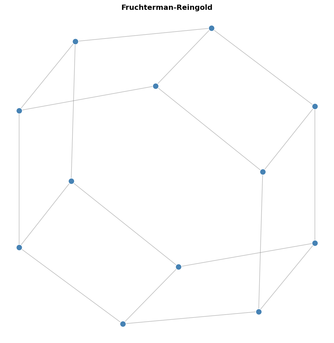
from graph_layout import FruchtermanReingoldLayout

layout = FruchtermanReingoldLayout(
    nodes=nodes,
    links=links,
    size=(800, 600),
    iterations=300,
    temperature=None,      # Auto-calculated if None
    cooling_factor=0.95,   # Temperature decay per iteration
)
layout.run()

Characteristics:

• Uses temperature/cooling schedule for simulated annealing

• Repulsive force: k^2 / d (inverse of distance)

• Attractive force: d^2 / k (quadratic with distance)

• Cython-accelerated for high performance

Complexity: O(n^2) per iteration (or O(n log n) with Barnes-Hut)

Parameters:

Parameter	Description	Default
iterations	Number of simulation steps	300
temperature	Initial max displacement	Auto
cooling_factor	Temperature multiplier per step	0.95
use_barnes_hut	Enable O(n log n) approximation	False
barnes_hut_theta	Accuracy vs speed (0=exact, 1=fast)	0.5

When to use Barnes-Hut:

• Graphs with 2000+ nodes

• When approximate positions are acceptable

• Real-time or interactive applications

---

Kamada-Kawai

Best for: Small to medium graphs where edge lengths should reflect graph-theoretic distances.

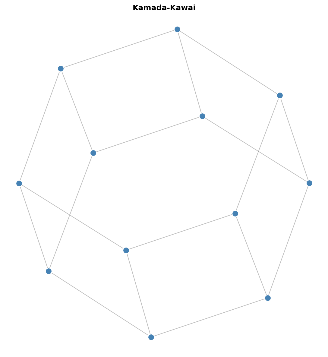
from graph_layout import KamadaKawaiLayout

layout = KamadaKawaiLayout(
    nodes=nodes,
    links=links,
    size=(800, 600),
    iterations=100,
)
layout.run()

Characteristics:

• Minimizes stress: deviation between geometric and graph-theoretic distances

• Computes all-pairs shortest paths (expensive for large graphs)

• Produces layouts where edge length correlates with path length

• Good for revealing graph structure

Complexity: O(n^3) for shortest paths + O(n^2) per iteration

Parameters:

Parameter	Description	Default
iterations	Number of optimization steps	100
epsilon	Convergence threshold	1e-4

Trade-offs:

• Higher quality than Fruchterman-Reingold for small graphs

• Much slower for large graphs due to all-pairs shortest paths

• Best limited to graphs under ~200 nodes

---

Spring Layout

Best for: Simple layouts, educational purposes, or as a baseline.

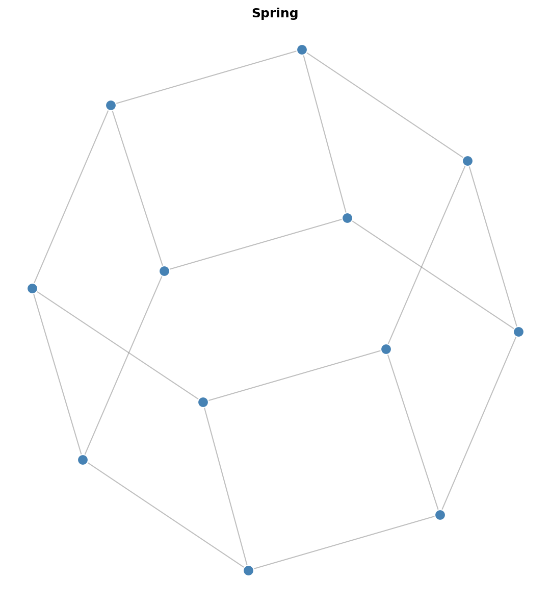
from graph_layout import SpringLayout

layout = SpringLayout(
    nodes=nodes,
    links=links,
    size=(800, 600),
    iterations=100,
    spring_length=100,   # Ideal edge length
    spring_strength=0.1, # Spring constant
    repulsion=1000,      # Repulsion strength
)
layout.run()

Characteristics:

• Simple Hooke's law springs for edges

• Coulomb-like repulsion between all node pairs

• No cooling schedule (constant forces)

• Easy to understand and modify

Complexity: O(n^2) per iteration

Parameters:

Parameter	Description	Default
iterations	Number of simulation steps	100
spring_length	Ideal edge length	100
spring_strength	Edge spring constant	0.1
repulsion	Node repulsion strength	1000
damping	Velocity damping factor	0.5

---

Constraint-Based Layout (Cola)

ColaLayoutAdapter

Best for: Layouts requiring constraints, overlap avoidance, or hierarchical grouping.

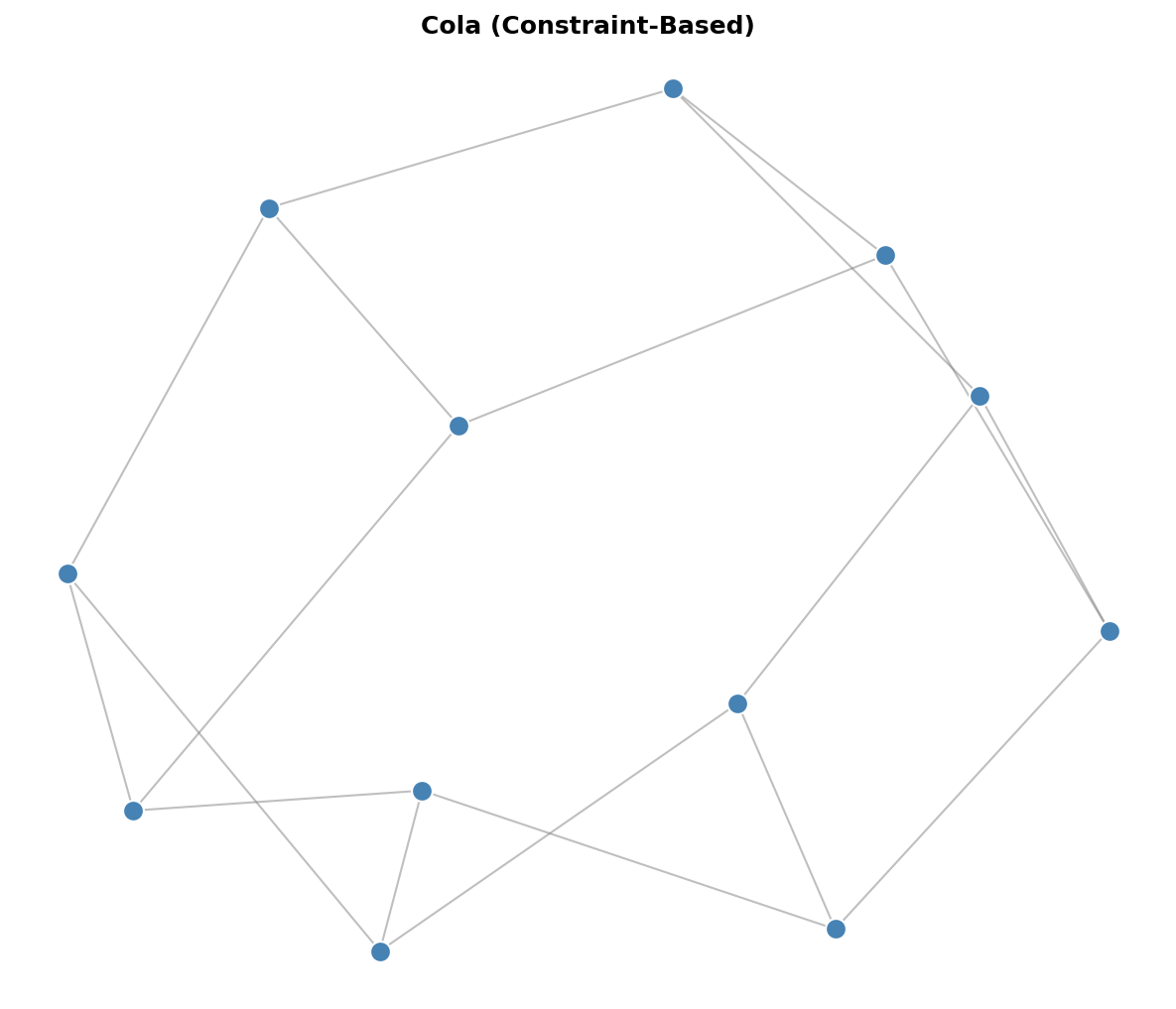
from graph_layout import ColaLayoutAdapter

layout = ColaLayoutAdapter(
    nodes=nodes,
    links=links,
    avoid_overlaps=True,
    link_distance=100,
    iterations=50,
)
layout.run()

Characteristics:

• Port of WebCola constraint-based layout

• VPSC solver for separation constraints

• Supports node overlap avoidance

• Hierarchical group containment

• Flow layouts (directional bias)

Complexity: O(n^2) per iteration + constraint solving overhead

Parameters:

Parameter	Description	Default
iterations	Layout iterations	50
link_distance	Ideal edge length (number or function)	100
avoid_overlaps	Prevent node overlap	False
handle_disconnected	Layout disconnected components	True
convergence_threshold	Stop when stress change below this	1e-4

Advanced Features:

# Separation constraints
from graph_layout.cola.linklengths import SeparationConstraint

constraint = SeparationConstraint(axis='x', left=0, right=1, gap=50)
layout = ColaLayoutAdapter(
    nodes=nodes,
    links=links,
    constraints=[constraint],
)

# Hierarchical groups
groups = [
    {'leaves': [0, 1, 2], 'padding': 10},
    {'leaves': [3, 4], 'padding': 10},
]
layout = ColaLayoutAdapter(
    nodes=nodes,
    links=links,
    groups=groups,
)

# Flow layout (left-to-right)
layout = ColaLayoutAdapter(
    nodes=nodes,
    links=links,
    flow_direction='x',  # or 'y' for top-to-bottom
)

---

Hierarchical Layouts

Sugiyama Layout

Best for: Directed acyclic graphs (DAGs), flowcharts, dependency graphs.

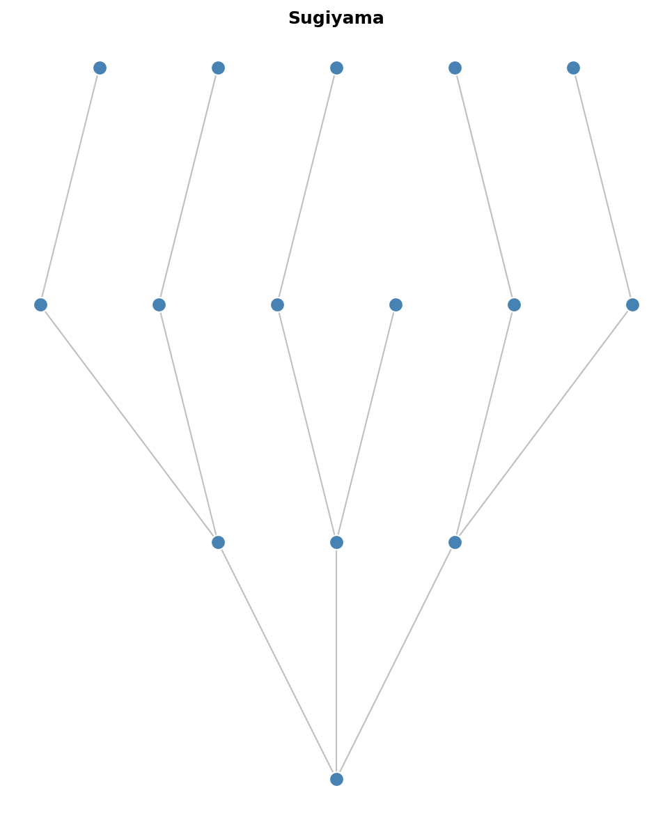
from graph_layout import SugiyamaLayout

layout = SugiyamaLayout(
    nodes=nodes,
    links=links,
    size=(800, 600),
    layer_separation=80,
    node_separation=50,
)
layout.run()

Characteristics:

• Assigns nodes to horizontal layers

• Minimizes edge crossings between layers

• Produces clean, readable hierarchical layouts

• Handles cycles by temporarily reversing edges

Complexity: O(n^2) for crossing minimization

Parameters:

Parameter	Description	Default
layer_separation	Vertical space between layers	80
node_separation	Horizontal space between nodes	50
direction	Layout direction ('TB', 'BT', 'LR', 'RL')	'TB'

---

Reingold-Tilford Layout

Best for: Trees and hierarchical structures.

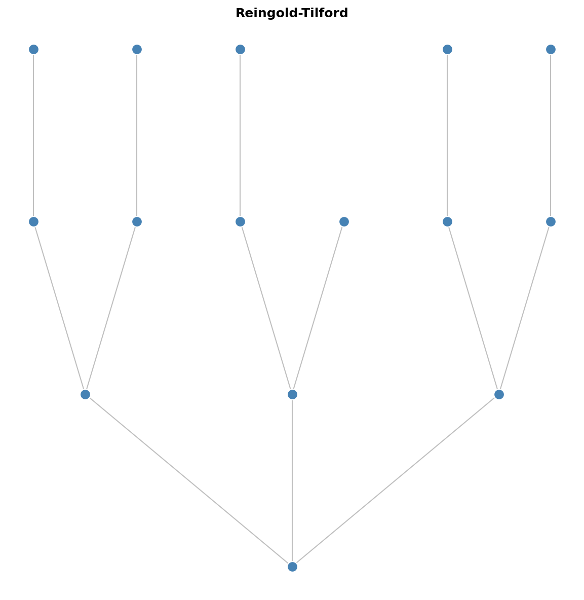
from graph_layout import ReingoldTilfordLayout

layout = ReingoldTilfordLayout(
    nodes=nodes,
    links=links,
    size=(800, 600),
    root=0,  # Root node index
)
layout.run()

Characteristics:

• Classic tree drawing algorithm

• Compact, balanced layouts

• Preserves tree structure clearly

• Requires a tree (single root, no cycles)

Complexity: O(n)

Parameters:

Parameter	Description	Default
root	Index of root node	0
node_separation	Horizontal space between siblings	1.0
level_separation	Vertical space between levels	1.0

---

Radial Tree Layout

Best for: Trees displayed as concentric circles from a central root.

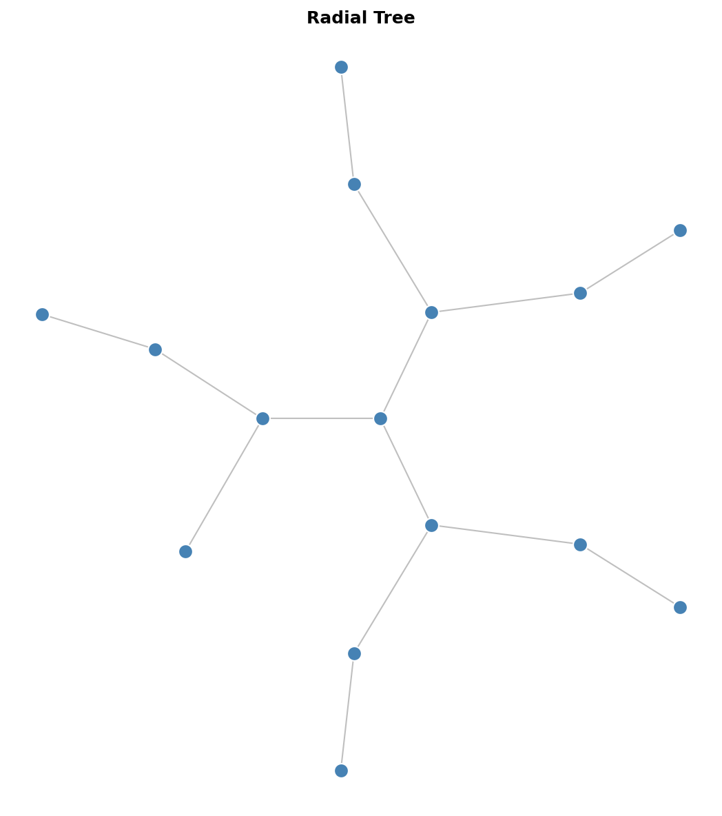
from graph_layout import RadialTreeLayout

layout = RadialTreeLayout(
    nodes=nodes,
    links=links,
    size=(800, 800),
    root=0,
)
layout.run()

Characteristics:

• Root at center, children in concentric rings

• Good for visualizing distance from root

• Works best with roughly balanced trees

Complexity: O(n)

Parameters:

Parameter	Description	Default
root	Index of root node	0
level_separation	Radial distance between levels	100

---

Circular Layouts

Circular Layout

Best for: Showing connectivity patterns, ring topologies, complete graphs.

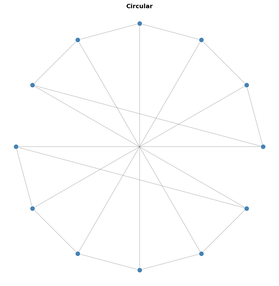
from graph_layout import CircularLayout

layout = CircularLayout(
    nodes=nodes,
    links=links,
    size=(800, 800),
    sort_by='degree',  # Order nodes by degree
)
layout.run()

Characteristics:

• All nodes placed on a single circle

• Simple and predictable

• Edge crossings can be minimized by node ordering

• Good for small to medium dense graphs

Complexity: O(n)

Parameters:

Parameter	Description	Default
sort_by	Node ordering ('none', 'degree', or callable)	'none'
start_angle	Starting angle in radians	0

---

Shell Layout

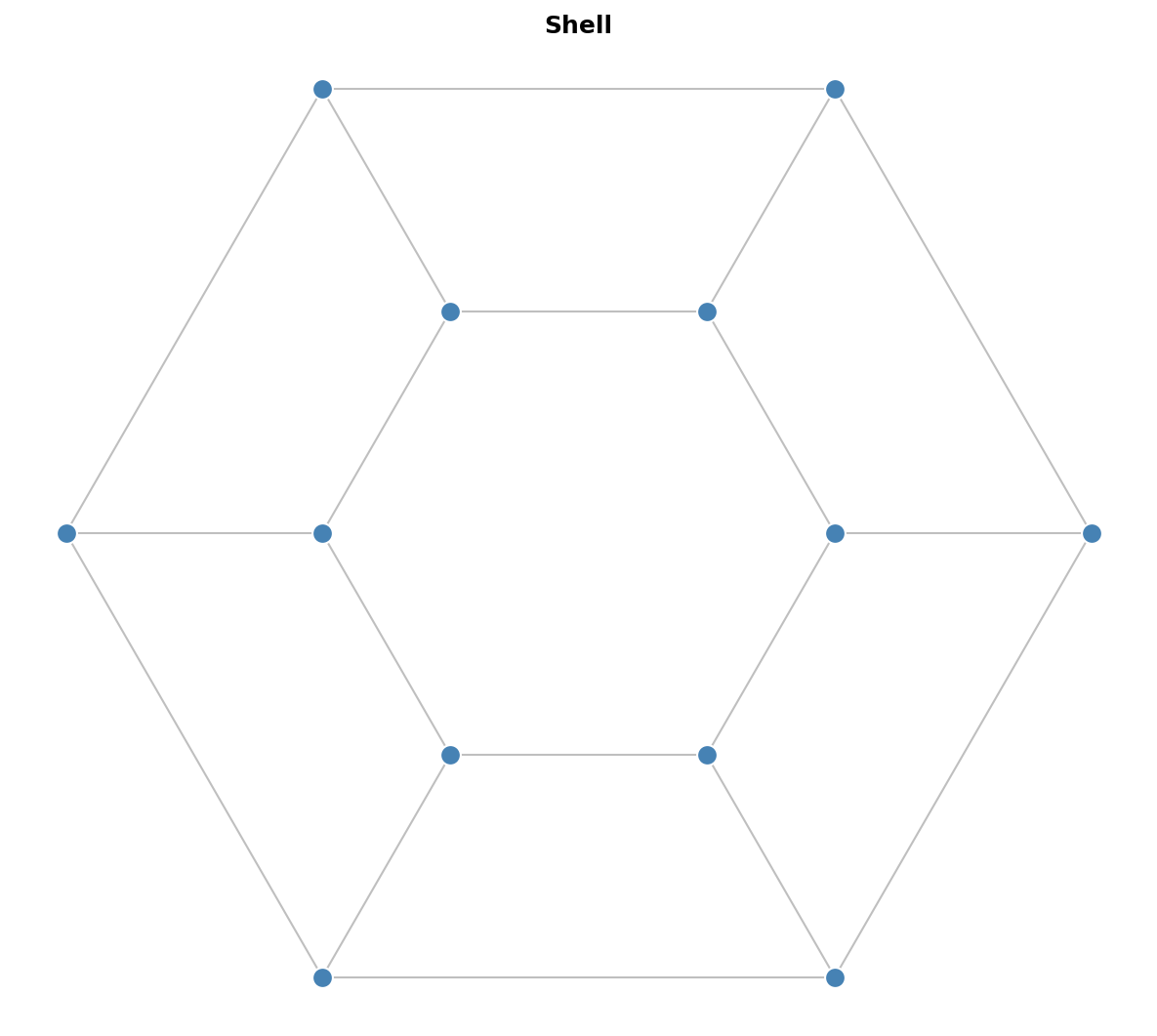
Best for: Grouped or stratified data, showing node importance.

from graph_layout import ShellLayout

# Automatic shells by degree
layout = ShellLayout(
    nodes=nodes,
    links=links,
    size=(800, 800),
    auto_shells=3,  # Number of concentric circles
)

# Manual shell assignment
layout = ShellLayout(
    nodes=nodes,
    links=links,
    shells=[[0, 1, 2], [3, 4, 5], [6, 7, 8]],  # Node indices per shell
)
layout.run()

Characteristics:

• Multiple concentric circles

• Can group nodes by degree or custom criteria

• Inner shells typically for important/central nodes

Complexity: O(n)

Parameters:

Parameter	Description	Default
shells	List of node index lists per shell	None
auto_shells	Auto-generate shells by degree	None

---

Spectral Layout

Spectral Layout

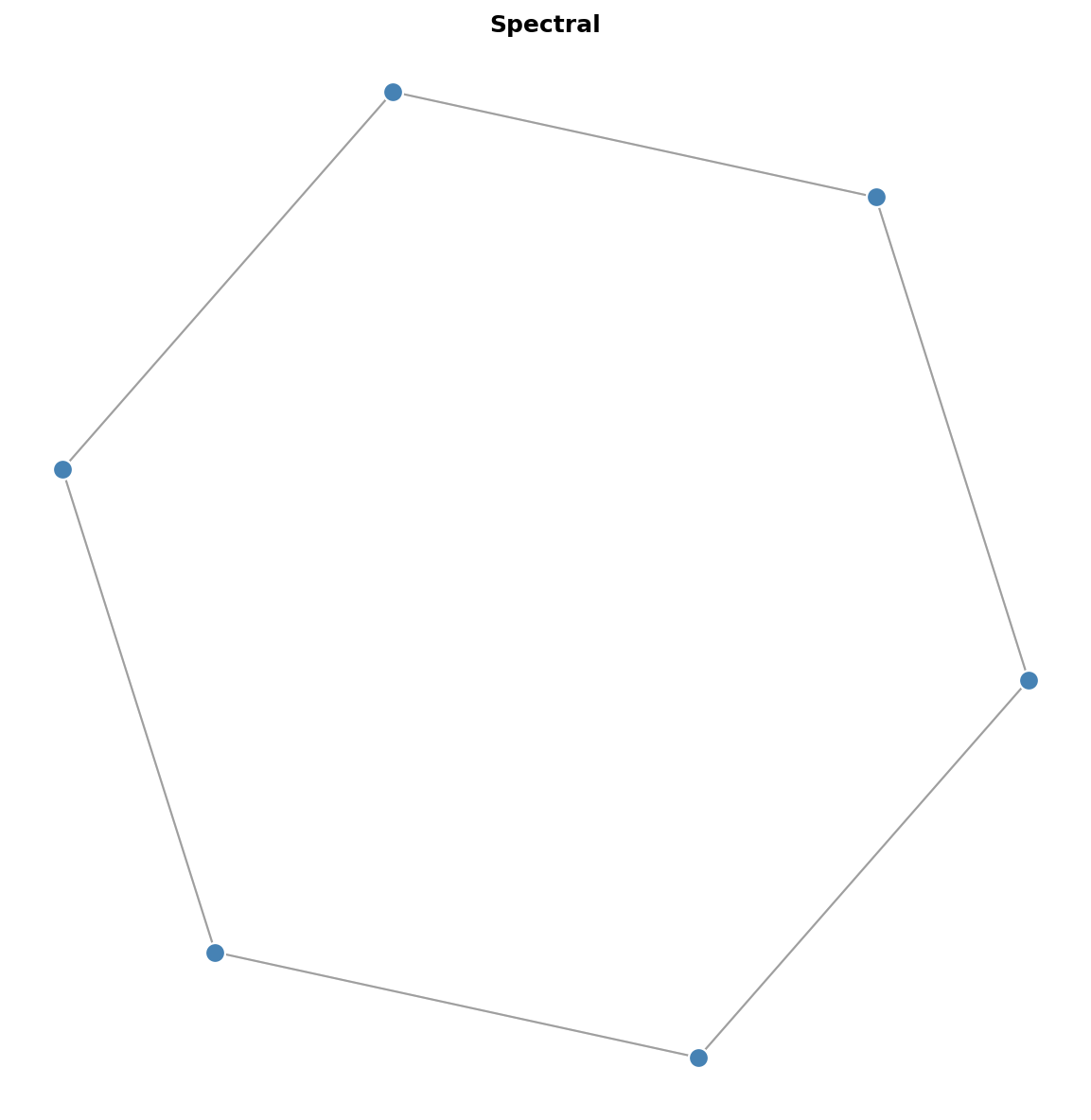
Best for: Revealing cluster structure, dimensionality reduction.

from graph_layout import SpectralLayout

layout = SpectralLayout(
    nodes=nodes,
    links=links,
    size=(800, 600),
    normalized=True,  # Use normalized Laplacian
)
layout.run()

Characteristics:

• Uses eigenvectors of the graph Laplacian matrix

• Positions based on graph's spectral properties

• Often reveals natural clustering

• Deterministic (same graph = same layout)

Complexity: O(n^3) for eigendecomposition

Parameters:

Parameter	Description	Default
normalized	Use normalized Laplacian	True
dimensions	Number of dimensions (2 or 3)	2

Trade-offs:

• Good at revealing structure but may not be visually optimal

• Expensive for large graphs

• Best for graphs under ~500 nodes

---

Planar Layouts

Crossing-free drawings of planar graphs. All draw any connected planar simple graph (>= 3 vertices) — internally triangulating and reusing one embedding/canonical-ordering substrate — and fall back to a circular placement for out-of-domain input, reporting the path taken via a used_* flag.

Schnyder / FPP / Tutte (straight-line)

Straight-line grid drawings. SchnyderLayout uses a realizer with vertex-count barycentric coordinates on the (n-1) x (n-1) grid; FPPLayout uses the de Fraysseix-Pach-Pollack shift method on the (2n-4) x (n-2) grid; TutteLayout fixes one face to a convex polygon and solves the barycentric equilibrium, giving convex faces for 3-connected planar graphs.

from graph_layout import SchnyderLayout

layout = SchnyderLayout(nodes=nodes, links=links, size=(800, 600))
layout.run()
assert layout.used_schnyder  # False if the graph was non-planar/disconnected

Use when: you want a compact, provably crossing-free drawing of a planar graph and prefer straight edges. Prefer Tutte for 3-connected graphs where convex faces matter.

Mixed-Model (visibility representation)

Draws vertices as horizontal bars and edges as bendless vertical segments attaching at distinct ports, spreading a high-degree vertex's edges across its bar for good angular resolution. Exposes vertex_bars and edge_routes.

Use when: the graph has high-degree vertices whose edges would be cramped in a straight-line drawing.

Planarization (non-planar input)

Draws a non-planar graph by replacing crossings with dummy vertices, then routing each edge as a polyline through its crossing points, so edges meet only at explicit crossing dots. Exposes crossings, crossing_count, and edge_routes.

Use when: the graph is non-planar but you still want a clean drawing with a small, explicit set of crossings.

---

Algorithm Comparison

Algorithm	Complexity	Best Graph Size	Constraints	Overlap Avoidance	Deterministic
Fruchterman-Reingold	O(n^2)/iter	Any	No	No	No
FR + Barnes-Hut	O(n log n)/iter	Large (2000+)	No	No	No
Kamada-Kawai	O(n^3) + O(n^2)/iter	Small (<200)	No	No	No
Spring	O(n^2)/iter	Small-Medium	No	No	No
Cola	O(n^2)/iter	Medium	Yes	Yes	No
Sugiyama	O(n^2)	Medium DAGs	Layering	Via spacing	Yes
Reingold-Tilford	O(n)	Any tree	Tree structure	Via spacing	Yes
Radial Tree	O(n)	Any tree	Tree structure	Via spacing	Yes
Circular	O(n)	Small-Medium	Circle	No	Yes
Shell	O(n)	Small-Medium	Concentric	No	Yes
Spectral	O(n^3)	Small (<500)	No	No	Yes
Schnyder / FPP	O(n^2)	Planar, any size	Planar	Grid points	Yes
Tutte	O(n^3) solve	3-connected planar	Planar	Convex faces	Yes
Mixed-Model	O(n^2)	Planar (esp. high-degree)	Planar	Bars/ports	Yes
Planarization	O((n+c)^2)	Non-planar	None	Explicit crossings	Yes

---

Decision Guide

Choose based on graph type

Is your graph a tree?
  Yes -> Reingold-Tilford (classic) or Radial Tree (centered)
  No  -> Continue...

Is your graph a DAG (directed, no cycles)?
  Yes -> Sugiyama (layered hierarchy)
  No  -> Continue...

Do you need constraints or overlap avoidance?
  Yes -> Cola
  No  -> Continue...

Is your graph large (>1000 nodes)?
  Yes -> Fruchterman-Reingold with Barnes-Hut
  No  -> Continue...

Do you want to reveal cluster structure?
  Yes -> Spectral
  No  -> Continue...

Do you want nodes on a circle?
  Yes -> Circular or Shell
  No  -> Fruchterman-Reingold (general purpose)

Choose based on requirements

Requirement	Recommended Algorithm
General-purpose, good aesthetics	Fruchterman-Reingold
Edge lengths reflect distances	Kamada-Kawai
Prevent node overlap	Cola
Hierarchical/layered display	Sugiyama
Tree visualization	Reingold-Tilford
Very large graphs (5000+)	FR + Barnes-Hut
Deterministic layout	Circular, Spectral, or hierarchical
Real-time/interactive	FR + Barnes-Hut or Spring
Reveal clustering	Spectral
Crossing-free planar drawing	Schnyder / FPP (straight-line), Tutte (convex)
Planar graph with high-degree nodes	Mixed-Model
Non-planar with few, explicit crossings	Planarization
Orthogonal (UML/ER/flowchart)	Kandinsky, GIOTTO

---

Performance Tips

1. Use Cython acceleration: Install from PyPI to get pre-built Cython extensions.

2. Enable Barnes-Hut for large graphs:

layout = FruchtermanReingoldLayout(
    nodes=nodes, links=links,
    use_barnes_hut=True,
    barnes_hut_theta=0.5,
)

1. Reduce iterations for previews: Use fewer iterations during interactive exploration, full iterations for final output.

2. Pre-filter large graphs: For very large graphs, consider filtering to show only important nodes/edges.

3. Use appropriate algorithms: Don't use O(n^3) algorithms (Kamada-Kawai, Spectral) on large graphs.